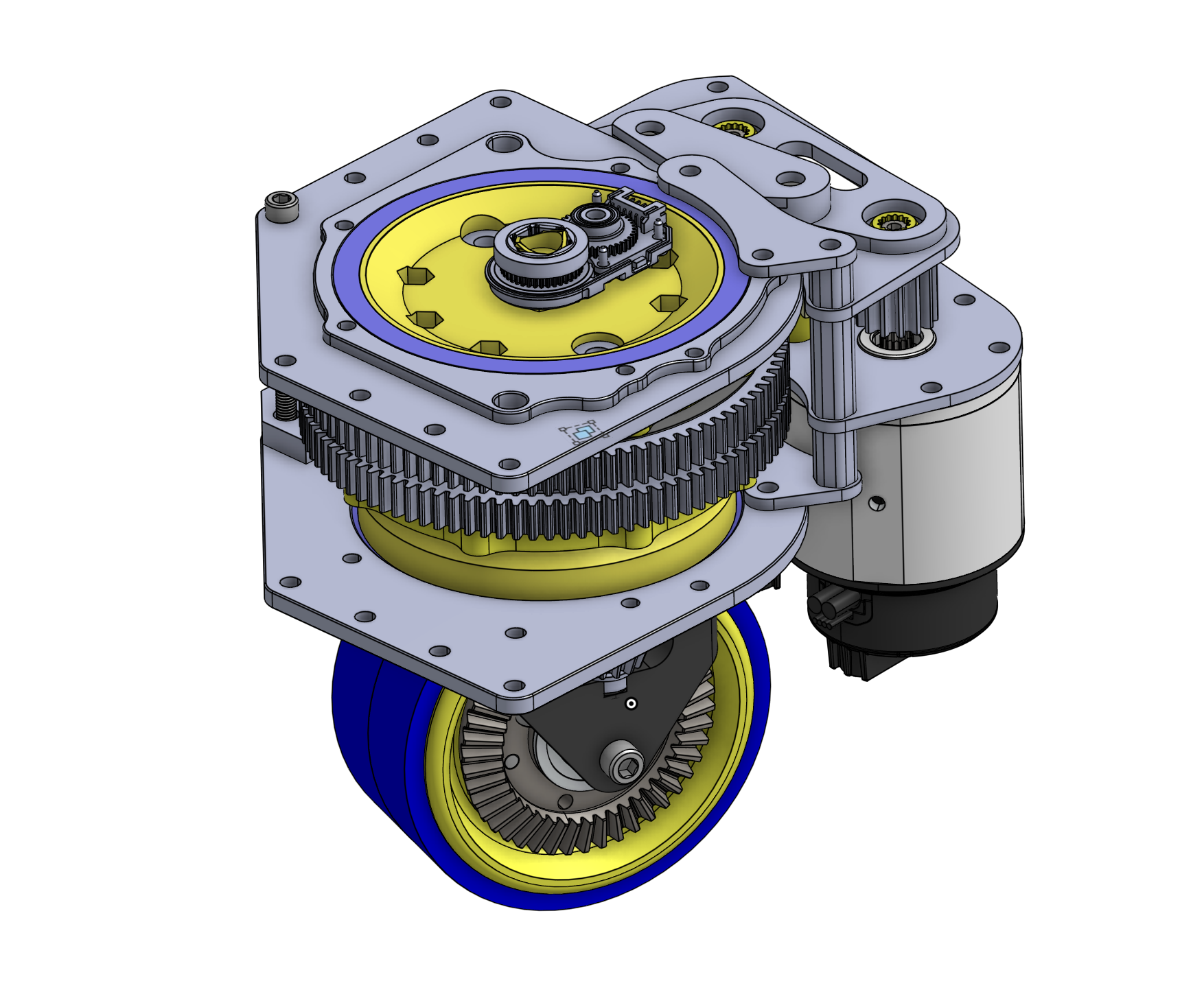
Differential Swerve Drive Module

Dynamic Model

Two motors control steering and wheel motion through differential coupling. Equal currents sum to steering torque, equal-and-opposite currents produce wheel torque. Current is the control input, assuming a fast inner current loop.

State vector

$$x = \begin{bmatrix} \theta_{\text{steer}} \\ \omega_{\text{steer}} \\ \omega_{\text{wheel}} \end{bmatrix}$$

Azimuth angle, azimuth rate, wheel angular velocity

Input vector

$$u = \begin{bmatrix} i_{\text{left}} \\ i_{\text{right}} \end{bmatrix}$$

Left and right motor currents (A), clamped to ±120 A

State-space equations $\dot{x} = Ax + Bu$

$$A = \begin{bmatrix} 0 & 1 & 0 \\ 0 & -\tfrac{f_s}{J_s} & 0 \\ 0 & 0 & -\tfrac{f_w}{J_w} \end{bmatrix}, \qquad B = \begin{bmatrix} 0 & 0 \\ \tfrac{k_t k_s}{J_s} & \tfrac{k_t k_s}{J_s} \\ \tfrac{k_t k_w}{J_w} & -\tfrac{k_t k_w}{J_w} \end{bmatrix}$$

Controllability matrix $\mathcal{C} = \begin{bmatrix}B & AB & A^2B\end{bmatrix}$ has rank 3, so the system is fully controllable.

My contribution

Derived the rotational dynamics, set up the full state-space model in MATLAB, verified controllability, tuned Q and R, computed the LQR gain, and ran all simulations. The mechanical assembly was a collaborative CAD effort with the team.

LQR Controller

LQR minimizes $J = \int_0^\infty \!\bigl[(x-x_d)^T Q\,(x-x_d) + u^T R\,u\bigr]\,dt$. Weights are chosen as inverse-squares of acceptable deviations: 0.15 rad on steering angle, 2.0 rad/s on each velocity state. Both motor currents are penalized equally.

Cost matrices

$$Q = \operatorname{diag}\!\left(\tfrac{1}{0.15^2},\ \tfrac{1}{2^2},\ \tfrac{1}{2^2}\right), \quad R = I_2$$

LQR gain $u = -K(x - x_d)$

$$K = \begin{bmatrix} 4.7140 & 0.3962 & 0.3536 \\ 4.7140 & 0.3962 & -0.3536 \end{bmatrix}$$

Closed-loop eigenvalues $\lambda(A_{\mathrm{cl}}) = \lambda(A - BK)$

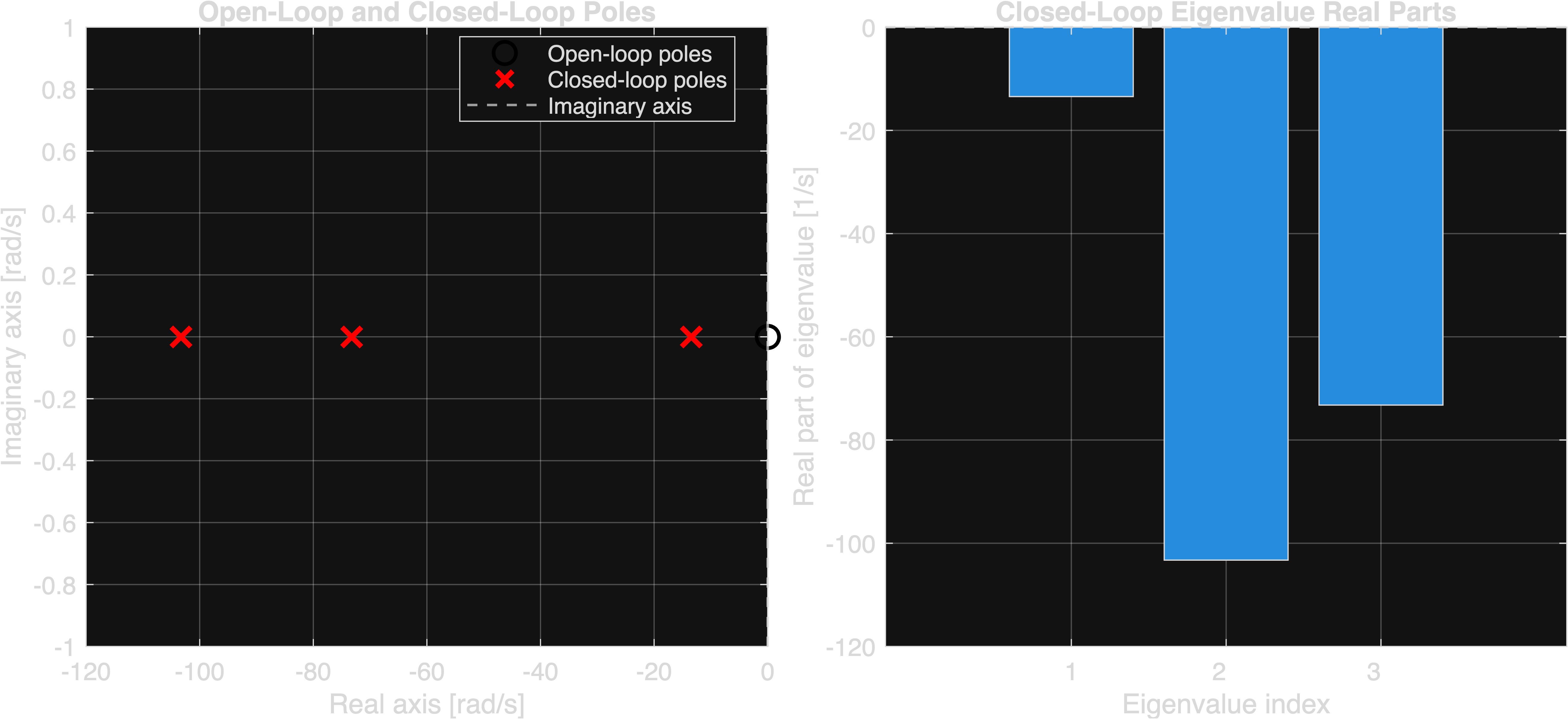
$$\lambda = \{-13.4459,\ -73.2257,\ -103.2715\}\ \mathrm{s^{-1}}$$

All eigenvalues are real and negative, the unsaturated continuous-time system is asymptotically stable.

Root Locus

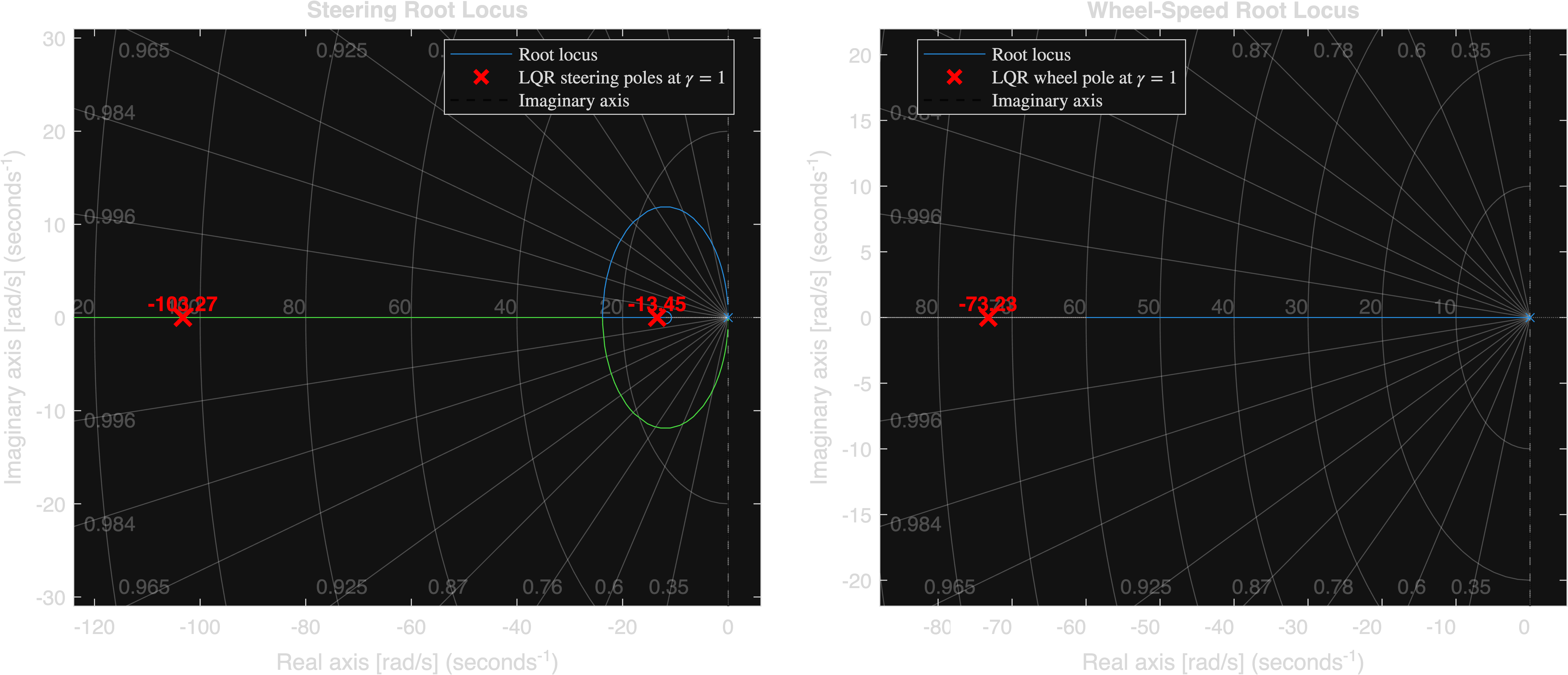
With two inputs a single classical root locus cannot be drawn for the full system, so the currents are decomposed into a common-mode steering channel and a differential wheel channel. The steering channel places poles at $-13.45$ and $-103.27\ \mathrm{s^{-1}}$; the wheel channel places a pole at $-73.23\ \mathrm{s^{-1}}$. Together these reproduce the three eigenvalues of the full closed-loop system. Red markers show the operating poles at the implemented LQR gain.

Closed-Loop Poles

All three closed-loop poles lie on the negative real axis. The $-13.45$ and $-103.27\ \mathrm{s^{-1}}$ poles govern steering dynamics. The $-73.23\ \mathrm{s^{-1}}$ pole governs wheel-speed dynamics.

Simulation Results

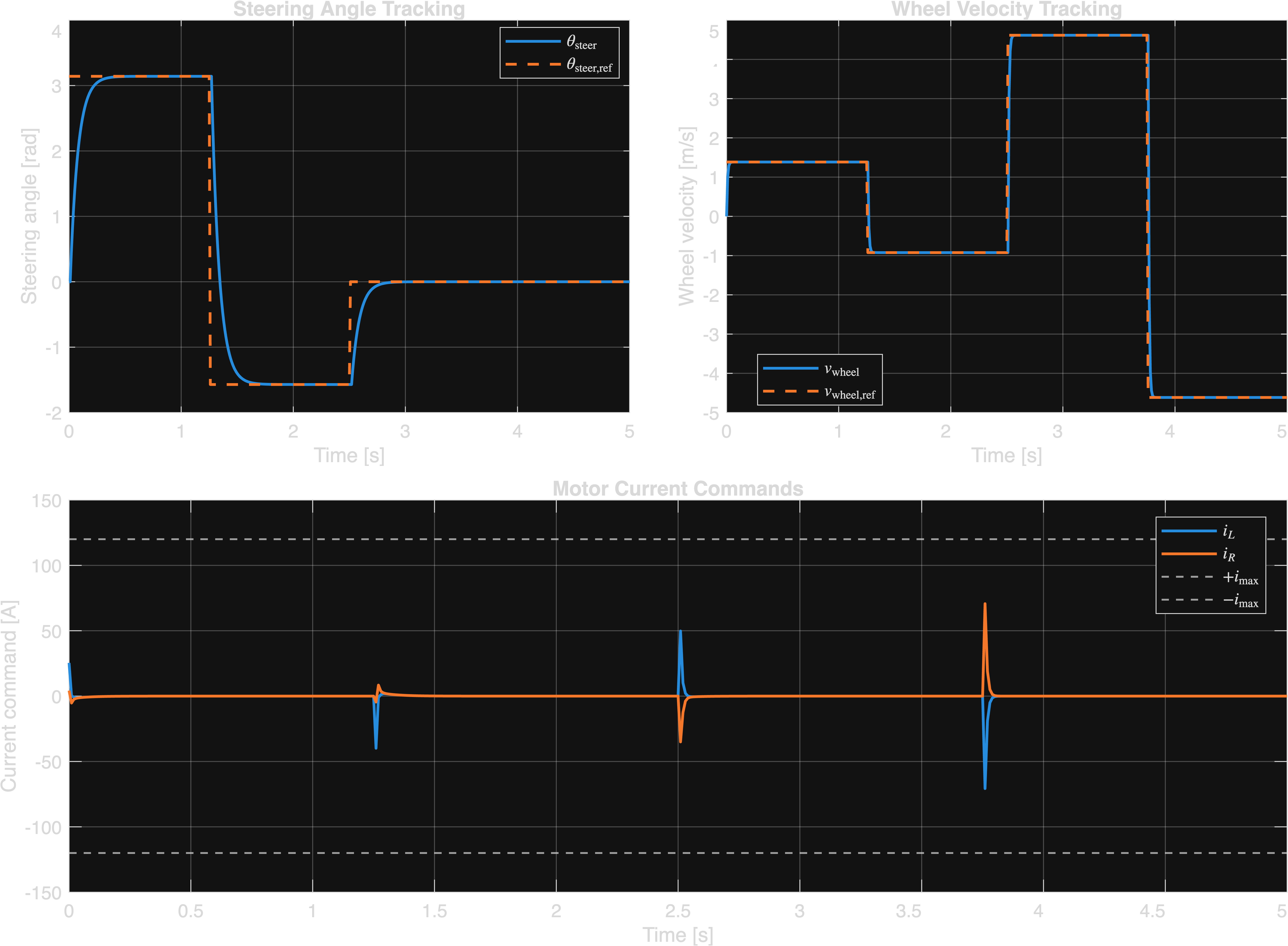
Step changes in azimuth angle (rad) and wheel velocity (m/s) over a 5 s run. The controller tracks four reference transitions: $\pi$ rad at 1.38 m/s, $-\pi/2$ rad at $-0.92$ m/s, then high-speed reversals to $\pm4.6$ m/s. Currents stay within the ±120 A limit, steady-state commands return near zero since the model has no friction or external load.

Simulation: steering angle, wheel velocity, motor currents

Module Test

Design Report CAD Files GitHub